Context

As hype is mounting around deep learning, do we still need to care about plain nearest neighbors search?

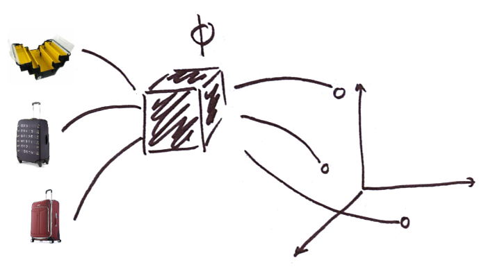
There is a recurring pattern in the deep learning pipelines: learn a representation for objects, and perform “simple” operations on the representations (that is, in the embedding space). And, as a matter of fact, one of the most useful operations is nearest neighbor search. For instance, product recommendation works with the following pipeline:

• learn a vector representation for products in dimension [latex]d[/latex]: for a product [latex]p[/latex], the representation is [latex]x = \Phi(p) \in \mathbb{R}^d[/latex] ; here [latex]\Phi[/latex] may be a deep neural network ;
• to compute a recommendation for a given user:
  • project the user in the same space, for instance using a combination of the products they’ve seen, and get [latex]u \in \mathbb{R}^d[/latex],
  • find the [latex]k[/latex] products closest to [latex]u[/latex]: [latex]R_k(u) = \mathcal{N}_k(u)[/latex], where [latex]\mathcal{N}_k(x)[/latex] are the [latex]k[/latex]-nearest neighbors of [latex]x[/latex]

 

Nearest neighbors are not dead. Instead, they’re a fundamental building block of modern AI systems. And they’re a fascinating, multi-faceted area of research. Faster, better algorithms for approximate nearest neighbor are introduced regularly, involving a wide range of techniques from computer science and machine learning for compressing and indexing data. In this post, I’ll explain a well-known but relatively little-talked-about phenomenon: hubness.

 

What is a hub?

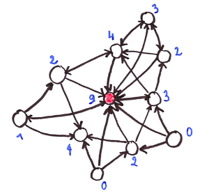
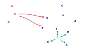
As the name suggests, this is an “attractor” point. You can get an intuition of it from the graph in the figure below: each node (point) is linked to its 3 nearest neighbors by an edge going from query node to the nearest neighbor. A hub is a node which tends to have much more in-going edges than the other nodes. Formally, we define [latex]N_k[/latex] the number of [latex]k[/latex]-occurrences of a node [latex]x[/latex], i.e. the number of points of which [latex]x[/latex] is in the [latex]k[/latex]-nearest neighbors list. As an example, the value of [latex]N_k[/latex] is written in blue next to each node in the figure. The node marked in red has a relatively large number of incoming edges and can be considered as a hub.

The presence of hubs is usually measured by computing the skewness of [latex]N_k[/latex], also known as the third standardized moment and defined as:

[latex] S_{N_k} = \frac{\mathbb{E}[(N_k – \mathbb{E}[N_k])^3]}{\sigma^3_{N_k}}.[/latex]

A random variable has positive skewness when its distribution is skewed to the right: there are a few points which have a large value. Visually, the curve is leaning to the left, since most points have low value. Here are a few examples of distributions with positive skewness:

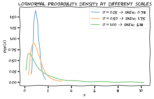
A high skewness is a sure sign of the presence of hubs. Beyond that, the actual skewness value is hard to interpret.

 

Why are there hubs?

When looking for [latex]k[/latex]-nearest neighbors, it seems natural that most points would be in the [latex]k[/latex]-occurrences of about [latex]k[/latex] points. In dimension 1, it’s pretty obvious that you can’t add more neighbors to a point [latex]x[/latex] without removing [latex]x[/latex] from the neighbor’s list of at least one of its previous neighbors – the new point has to come in between at some point. You can check it in dimension 2 as well: there’s a threshold at which you can’t add more neighbors to [latex]x[/latex] without removing [latex]x[/latex] from another point’s [latex]k[/latex]-occurrences…

Why and when hubness arises has been studied fairly recently in the literature, after the phenomenon was observed in a number of nearest neighbors applications, such as recommender systems. In a comprehensive study, Radovanović et al. showed that hubs arise as a consequence of the curse of dimensionality, as well as the presence of some centrality in the data.

High-dimensional spaces and the curse of dimensionality

The curse of dimensionality shows up in different ways. Let’s take a simple example to understand why there is such a thing as the curse of dimensionality.

Let [latex]V_d(r)[/latex] be the volume of a sphere of radius [latex]r[/latex] in dimension [latex]d[/latex]. It’s volume is proportional to [latex]r^d[/latex]. You know it already in dimension 2: it’s the surface of a circle, ie [latex]V_2(r) = \pi r^2[/latex] ; and in dimension 3, [latex]V_3(r) = \frac{4}{3}\pi r^3[/latex]. So, more generally, [latex]V_d(r) = \alpha_d r^d[/latex].

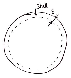
Now let’s compute the volume [latex]S_d(\epsilon)[/latex] of a shell of thickness [latex]\epsilon[/latex] on this sphere. This is the total volume of the sphere, minus the volume of the inside, ie for [latex]r=1[/latex]:

[latex]S_d(\epsilon) = V_d(1) – V_d(1-\epsilon) = \alpha_d(1 – (1 – \epsilon)^d).[/latex]

So the ratio [latex]S_d(\epsilon) / V_d(1)[/latex] tends to [latex]1[/latex] when [latex]d[/latex] grows to infinity. The figure below shows a plot of the normalized volume of the shell [latex]S_d(\epsilon)/ V_d(1)[/latex] for a few values of [latex]\epsilon[/latex] below (showing what fraction of the sphere is occupied by the shell). If the shell is 10% the length of the radius, at dimension 200 and even below that, the volume of the shell is the volume of the sphere. What? Yes! [latex]S_d(\epsilon) / V_d(1)[/latex] is so close to 1, both volumes are almost indistinguishable.

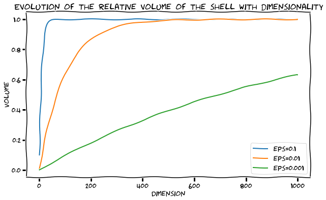
What does that imply? If you take points uniformly at random within a hypersphere of dimension d and radius 1, it’s very likely that most of these points will lie on the shell of the sphere. Don’t trust your intuitions when you work in high dimensions.

Concentration of distances is a related phenomenon: in high dimension, the distances between any two points are all similar. More formally, it has been proved that the expectation of the Euclidean norm of i.i.d random vectors grow with the square root of the dimension, whereas its variance tends towards a constant when the dimension tends to infinity. As the Euclidean distance is the norm of the difference of such 2 vectors, it exhibits the same behavior. Since all distances grow, but not their variance, it becomes hard to distinguish which point is closer to which. In certain situations, you can prove that the difference between the distances to closest and farthest points to an anchor point tends towards 0… so that you can’t expect nearest neighbor algorithms to distinguish efficiently which points are actually closer. The concentration of distances is a well-studied aspect of the curse of dimensionality.

Hubness is a related but distinct aspect of the curse. When dimension increases, all distances grow. But if A is a point closer to the data mean that an average point B, it turns out that the distance from A to any point grows more slowly than the distance from B to any point. This is one of the main points of Radovanović et al., who prove that central points thus become hubs in high dimension. That’s what we’ll refer to as the “classical hubness”.

Classical hubness examples

Radovanović et al. show the hubness phenomenon empirically, showing increase skewness of the distribution of [latex]N_k(x)[/latex] when the dimension [latex]d[/latex] increases.

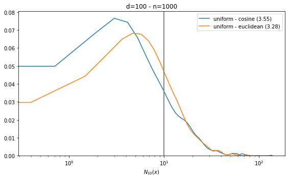
Their experiments are easy to reproduce. We can observe hubness on a number of distributions, but for simplicity, we only show results for the uniform distribution in the figure below. Note the difference: in small dimension (eg d=5), the distribution is peaked at [latex]k[/latex]. In that case, there is no hubness, as confirmed by the skewness value (in brackets, in the legend). The results are similar for 2 commonly used distances, Euclidean and cosine. The x-axis is in log scale on the second plot for readability.

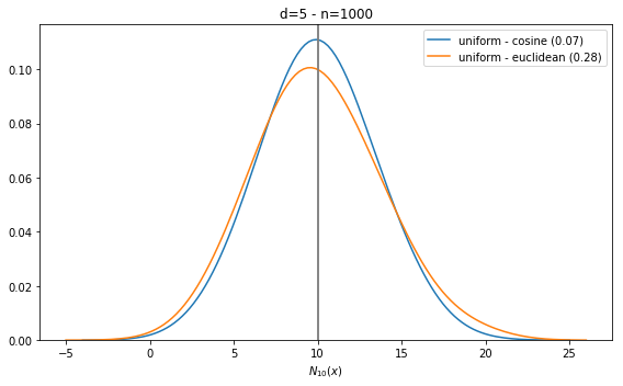
There are rare cases where there is no hubness even in high dimension, for instance, when the cosine distance is used with normally distributed data. This is because in that unusual case, there is no _central position_ in the data. That doesn’t really happen with real data.

Another case of hubness

One way of doing cross-advertiser recommendation is to project all products in a common embedding space (eg advertiser A in red, advertiser B in blue below). When a user has visited advertiser A, you can use the products seen to represent the user and find nearest products from advertiser B. However, there is a catch: if advertisers A and B correspond to two different clusters in the embedding space, the same products will tend to always appear in the recommendation list. This is another kind of hubness effect, which is independent of dimension or data centrality. We dub this phenomenon cross-cluster hubness.

This kind of hubness arises in undesirable situations where the query actually comes from a totally different distribution than the indexed products.

As you could expect, hubness is very correlated to a coverage metric, which would measure the number of products from B which appear in [latex]k[/latex]-NN lists, when querying all products from A, divided by the total number of products from B. It can be shown that coverage is negatively correlated with skewness, ie whenever there are hubs, fewer products are selected by the recommender system. This metric has the advantage over skewness of being easy to interpret.

 

What are the consequences?

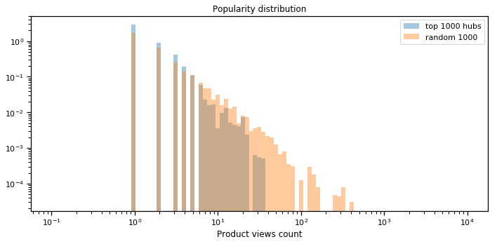
A direct and simple consequence of hubness is that some products appear much more often than others in a recommendation. It’s unlikely to be a good feature: it decreases diversity, and it might miss better recommendations which are farther in terms of the distance used. Indeed, popular products are usually good recommendations, and we found that hubs aren’t popular products, but rather less likely to be popular than a random product, as shown in the figure below, showing the distribution of a number of views for hubs vs. any product.

Worse: cross-advertiser nearest neighbors may sometimes give dramatically low coverage, in the degenerate case when query and target advertisers don’t match well in the computed representation space. Being able to detect and mitigate these situations is key to improving the quality of the system.

A number of heuristics have been proposed to mitigate this effect in various applications. As a well-defined research topic, it is relatively young though: Feldbauer and Flexer recently published a survey of the hubness reduction techniques. The authors performed an analysis on 50 datasets, analyzing hubness reduction and [latex]k[/latex]-NN classification accuracy. They show that hubness reduction is especially useful to increase classification accuracy for data sets with high hubness. Hubness reduction methods usually rely on computing reverse nearest neighbors, or (equivalently) using precomputed distances in the [latex]k[/latex]-NN graph. For instance, a simple but powerful method is a simplified version of Non-iterative contextual dissimilarity measure (taken from Schnitzer et al.), which works like this:

• for each data point [latex]x[/latex], compute a scaling parameter [latex]\mu_x[/latex] as the average distance from [latex]x[/latex] to its [latex]k[/latex] nearest neighbors,
• reweight distances: [latex]\text{NICDM}(d(x, y)) = \frac{d(x, y)}{\mu_x\mu_y}[/latex].

Most other methods can be seen as variants upon this idea: using another kind of reweighting functions, and other kinds of scaling parameters.

Many open questions remain for us: can we use these hubness reduction methods to effectively improve recommendation at our scale? How is it going to generalize to the special case of cross-cluster hubs?

---

Post written by:

References

• Radovanović, Miloš, Alexandros Nanopoulos, and Mirjana Ivanović. “Hubs in space: Popular nearest neighbors in high-dimensional data.” Journal of Machine Learning Research 11.Sep (2010): 2487-2531.
• Schnitzer, Dominik, et al. “Local and global scaling reduce hubs in space.” Journal of Machine Learning Research 13.Oct (2012): 2871-2902.
• Feldbauer, Roman, and Arthur Flexer. “A comprehensive empirical comparison of hubness reduction in high-dimensional spaces.” Knowledge and Information Systems (2018): 1-30.