Introduction
Every two years, the French Society of Statistiques (SFdS) organizes a conference on a statistical topic for a week.
This year was devoted to Causality, starting from philosophical introduction to practical sessions on Bayesian networks.
As a researcher in causal advertising, I am deeply interested on the matter. Here are my key learnings.
I joined as a R&D researcher to discuss causality is part of my job. Find here my key learnings.
A bit of history of causality in philosophy and sciences
This is extract from Isabelle Drouet lecture
How to define “causality”? Back in the 18th, Hume defined the efficient causality as a mental capacity, meaning the ability to link a cause to its effect.
Quite simply, he followed the regularist approach, meaning that:
- Causes and effects are contiguous,
- Causes appear before their effects,
- Causes are always followed by their effects.
Generic causality as described here is to be opposed to singularity causality. And all it takes is a single counterexample to annul the causality link.
More recently, in 1974, Machies defined the INUS conditions : Insufficient but Necessary to Unnecessary but Sufficient. What does this mean?
For example, A and B are sufficient but unnecessary (only one of them is necessary).
But A is composed of A1 and A2 and B is composed of B1 and B2. A1 and A2 are necessary to form A but insufficient alone because both A1 and A2 are needed. The same happens to B1 and B2. [EXAMPLE]
What’s important to bear in mind was that up to the 20th century, the causality was mainly linked to determinism and necessity.
Yet with the beginning of statistics, the notion of causality turns up to be considered too rigid and therefore rejected. One of its striking example is Russell, in On The Notion of Cause: ”The law of causality, I believe, like much that passes muster among philosophers is a relic of a bygone age, surviving, like the monarchy, only because it is erroneously supposed to do no harm” (1979).
In 1970, Suppes defends that:
A Cause increases the probability of its effect and happens before.
Also A is a cause of B if P(A|B)>P(A) and P(B|A)>P(B) and there is no C such that P(A|C)>P(A) and P(B|C)>P(B) and P(A,B|C) = P(A|C)P(B|C).
A few years later in 1979, Cartwright adds the notion of sub-population: the probability increase had to stay true even in sub-population.
Counterfactual Theories
Yet some counterfactual theories are to be linked. The approaches become singular instead of general.
Basic idea: c causes e if and only if
Lewis defined two different worlds, one in which c happens and the other one in which it does not.
Interventionist Approach
Last approach is that of interventionist.
X causes Y if we can modify Y by intervening on X.
This approach is not in conflict with statistics and probabilities. It can be formalized by causal graphs and structural equations.
On the levels of Causality
This is a sum up on the Introduction to Causality made by Antoine Chambaz and Vivian Viallon.
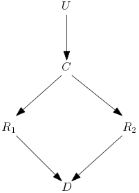
Let’s take the example of a causal draft with the execution platoon.
The judge can order to kill the prisoner, U is 1 if the order is given else 0.
Then the commander gives the order simultaneously at the two soldiers to kill the prisoner, C is 1 if the order is given else 0.
The two soldiers fire when they receive the order from their commander, R1 and R2 are 1 if they fired, else 0.
D is 1 if the prisoner is dead and else 0 (we assume that the two soldiers never miss their target and that the prisoner cannot die but from a gunshot).

Figure 1 Causal Graph
Pearl defines three level of causality.
- Association:
Observation level.
If D is true, is U true? Yes, because if D then the soldiers received order by the commander which received it from the judge.
If R1 is true, is R2 true? Yes, because the two soldiers obey to the same order.
- Intervention:
In that level, we can do intervention.
What will happen if R1 fires even without C? D is true, but this cannot happen without our intervention.
- Counterfactual:
Use of imagination not only action.
What would had happened if D but R1 did not fire? R2 and D would stay true.
The ideal setting for causal inference is to know how each individual would react to each treatment.
At an individual level Y1 – Y0 and at a population level E(Y1 – Y0) = P(Y1) – P(Y0).
Usually theses data are not given, therefore we need to set up hypotheses:
- coherence: When intervention do(a=a), Y= Ya (not always the case when individuals interact with each other).
- ignorability: Ya is independent of A.
- conditional ignorability: Ya is independent of A|W where W is the rest of the system.
Average causal effect (ACE), ACE = E(Y1) – E(Y0), with the ignorability hypothesis we can write ACE = E(Y1|A=1) – E(Y0|A=0) and the coherence hypothesis gives us ACE = E(Y|A=1) – E(Y|A=0).
Structural Causal Models
This causal draft is a Directed Acylic Graph (DAG). In that case, the hypothesis contains the coherence and conditional ignorability hypotheses.

Figure 2 Causal Graph with intervention
On the graph UA and UY are exogenous variables, noise that we cannot observe.
A and Y are endogenous variables that we observe.
The corresponding function equations are:
A = fA(UA)
Y = fY(UY,A)
After an intervention on A it becomes:
Ya = fY(UY,a)
NB: Functional equations cannot be inverted to express UA in function of A, they are not arithmetic equations.

Figure 3 Causal Graph with mediator (left) and confounding (right)
With the confounding variable, an intervention will not lead to Ya independent of A but to Ya independent of A conditioning on C, the conditional ignorability.
Identifiability under causal models
Causal model is M= (V,U,F) with:
- V representing endogenous variables
- U representing exogenous variables
- F representing functional equations
We consider a causal model to be Markovian when exogenous variables are independent.
How to identify a causal effect? We consider if is identifiable if it is possible to express it with observable variables.
In that case, a set of d-separable criteria allow us to figure out if two sets of variables are independent, given a third set of variables.
Pearl 3 rules of do-calculus allows to identify the effect of an intervention.
The back-door criterion identifies the set of variables on which to make the intervention.
The front-door criterion is a sufficient but not necessary criterion for identifiability.
On the Simpson Paradox
The Simpson Paradox can arise when a confounding affects both the cause and the effect.
| Treatment A | Treatment B | |
| Small stones | 93% (81/87) | 87% (234/270) |
| Large stones | 73% (192/263) | 69% (55/80) |
| Both | 78% (273/350) | 83% (289/350) |
For example, in the kidney stone instance of the paradox.
Treatment A works better on the sub-population with small stones as well as on the sub-population with large stones.
However, in the global population, treatment B seems better.
The paradox arises because treatments are not chosen at random.
When a case is difficult, when the stone is large, the doctor gives treatment A.
On the contrary when the case is easy, the doctor gives the treatment B.
Dynamical approach to causality
This is an extract from the talk presented by Daniel Commenges
We notice two approaches:
- Directly estimate marginal effects with randomization
- Estimate conditional effects and deduce marginal effects
Instead of counterfactual approach (what would have happened if B instead of A) consider different probability laws.
This approach represents phenomena with a stochastic process in continuous time.
We came across interesting Mechanical models like Voltera or the equilibrium between hosts and pathogens.
Let’s take one of them: the AIDS example.
There are two equilibria, one without infection, and one if individual is infected but the reproductive factor is below 1.
Because of individual variations the reproductive factor changes.
There are a lot of studies to estimate it and to give the minimal drug quantity to fall below 1 with minimal secondary effects.
Causality and Learning
This is an extract from Léon Bottou’s presentation.
Causality applied to the reserve price choice for ads on a search engine.
Intervention consists in changing the distribution of the reserve price.
But we only have old data, so we need to use Counterfactual Expectation (Importance Sampling and Monte Carlo estimation) to estimate the potential outcome under a different probability law.
Importance sampling (IPS) is unbiased but has high variance if the domains of the two distributions do not overlap enough.
Use of clipping: samples with a huge IPS weight are rejected.
We can reduce the variance by changing the reweighted variable. For example, the reserve price is not important as long as the ad shown is the same. So instead of doing IPS on the reserve price we can do IPS on the shown ad. This reduce the variance.
We can also use sequential learning by testing a small change and learn again and repeat.
When we perturb a system, it reaches a new equilibrium hard to predict.
Also, problems of multiple teams: examples of two teams working on different objectives but the experiments of one bias entirely the conclusions of the second one.
In conclusion, it was super interesting to learn about causal advertising in other domains like health. I really appreciate that Criteo provides each researcher with the opportunity to attend 2 national conferences per year as well as an international one.
Hope you learnt some things as well!
Amelie Heliou
Researcher AI Lab

