
At Criteo AI Lab, we are using more and more complex machine learning (ML) models every day. This means that we have many more hyper-parameters to tune. A lot of ML model tuning used to be done by hand and accelerated by domain knowledge. This meant that a team of experts was dedicated to a little portfolio of models, with a lot of menial work involved. Automated hyper-parameter tuning brings a solution to these problems.

So, where is the optimum?
Hyper-parameter tuning refers to the automatic optimization of the hyper-parameters of a ML model. Hyper-parameters are all the parameters of a model which are not updated during the learning and are used to configure either the model (e.g. size of the hashing space, number of decisions trees and their depth, number of layers of a deep neural network, etc.) or the algorithm used to lower the cost function (learning rate for gradient descent algorithm, etc.). This idea can be pushed further to include the optimization algorithm (for neural nets: stochastic gradient descent, Adam, RmsProp, etc.) as an hyper-parameter. The last step is to include the type of model itself (logistic regression, ensembles of trees, neural nets) and also the features which are fed into the algorithm, but here we are venturing in the realm of autoML, which promises to put the human out of the loop of ML model design.
Conceptually, hyper-parameter tuning is just an optimization loop on top of ML model learning to find the set of hyper-parameters leading to the lowest error on the validation set. Thus, a validation set has to be set apart, and a loss has to be defined. As usual, the cost function needs to be a scalar, as multi-objective optimization is out of the reach for this article.
This outer-loop optimization is done on a ML system, and this has two implications. First, the evaluation of the function is very costly, as it entails learning a model (which can take hours if not days on a large scale computing cluster) and evaluating its performance on a validation set. Secondly, the model is evaluated on a validation set, which is a substitute to get the expected performance on the true distribution of the data (which leads to the generalization error). The performance of the model is evaluated with some error, and thus there is no point in finding the true optimum with a high precision.
As opposed to the optimization algorithm of the ML model, no gradient is computed, so the hyper-parameter optimization algorithm cannot rely on it to lower the validation error. Instead, it must blindly try a new configuration in the search space or make an educated guess of where the most interesting configuration might be. It is why these optimizers are called black-box optimizers. There is an active field of research on getting the gradient of the model with respect to the hyper-parameters (for instance, see [4] and [10]), but to the best of our knowledge, the methods proposed are not mature enough to be used in real world problems with large models.
Now, we will review the main types of algorithm used for hyper-parameter optimization.
Classes of algorithms
The hyper-parameter optimization algorithms can be separated into three main categories, namely exhaustive search of the space, surrogate models and finally some algorithms mixing some ideas of the two previous categories and specifically dedicated to hyper-parameters tuning.
For all these algorithms, a search space has to be defined beforehand, setting bounds for all the hyper-parameters, and also adding some prior knowledge on them (like setting a non-uniform distribution for the search, e.g. learning rates have to be searched on a log distribution).
Exhaustive search of the search space
Grid search
The search space of each hyper-parameter is discretized, and the total search space is discretized as the Cartesian products of them. Then, the algorithm launches a learning for each of the hyper-parameter configurations, and selects the best at the end. It is an embarrassingly parallel problem (provided one has the computing power needed to train several models at the same time) but suffers from the curse of dimensionality (the number of configurations to try is exponential with regards to the number of hyper-parameters to be optimized).
Random search
A variation of the previous algorithm, which randomly samples the search space instead of discretizing it with a Cartesian grid. The algorithm has no end. Instead a time budget has to be specified (in other words, a number of trials). This algorithm suffers likewise from the curse of dimensionality to reach a preset fixed sampling density. One of the advantages of random search is that if two hyper-parameters are little correlated, random search enables to find more precisely the optima of each parameter, as shown on the figure below.
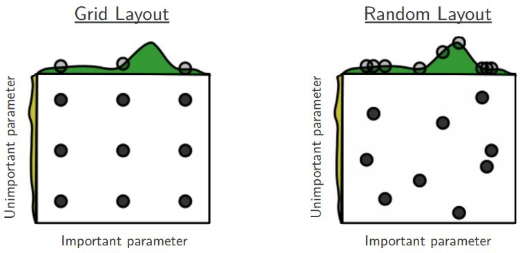
Benefits of using random search against grid search. Image taken from [2]
Random search has proven to be particularly effective, especially if the search space is not cubic, i.e. if some hyper-parameters are given a much greater range of variation than others. See [2] for some explanations.
Using purely random sampling for picking the next next hyper-parameter sample can give a non-uniform sampling density of the search space. Low-discrepancy sequences can be used to ensure a more uniform sampling (and hence better bounds on the finding of the global minimum) (see [2] for more details).
Random search and grid search are an attractive first option for optimization. They are very easy to code, can be run in parallel and they do not need any form of tuning. Their drawback is that there is no guarantee of finding a local minimum to some precision except if the search space is thoroughly sampled. This does not pose any problem if the model is very fast to run and the number of hyper-parameters is low. If the model takes a significant time to run using a lot of computational resources, random or grid search are inefficient as they do not use the information gained by all the previous tries.
Use of a surrogate model
A surrogate model of the validation loss as a function of the hyper-parameters can be fit to the previous tries, and tell where the local minimum might be. These methods are called Sequential Model-Based Optimization (SMBO).
Bayesian optimization
Bayesian optimization can be easily explained when looking at Gaussian process regression (also known as kriging). Gaussian processes are stochastic functions which, when sampled on k random points, follow a multivariate Gaussian distribution. See [11] for a full review. In more simple words, Gaussian processes are the generalization of multivariate random distributions to function (i.e. of infinite dimensions). One key point of Gaussian processes is that they are completely defined by their second-order statistics. If f is a Gaussian process, and x1, x2 are two points (think hyper-parameter configurations), then, assuming f has zero mean and is stationary (i.e. the variance of f does not depend on space)
Cov(f(x1), f(x2)) = k(x2 – x1)
Here, k is a kernel function which depends only on the vector distance between the two points. Several functions can be used as a kernel, such as the Gaussian function (also called squared exponential).
Gaussian process regression (also called kriging) means adding to the prior (shape of the kernel, etc.) the additional information of the already sampled points. In other words, it tries to fit the response surface by a Gaussian process with a prior covariance (i.e. kernel function). The mean of the Gaussian process gives the approximate response, but there is also much insight to be gained by looking at the predicted variance. One chooses then an acquisition function (a function of the Gaussian process), which will enable the selection of the next point to sample in the hyper-parameter space. There are many ways to define such a function.
For instance, one can use the expected improvement function (EI) as an acquisition function. It is defined as EI(x) = E[max(0, f(x) – f(x*))], where f is the Gaussian process fitting the response surface, x the hyper-parameter and x* the best hyper-parameter so far. As f is probabilistic, we need to take the expectation of this quantity. Another popular acquisition function is the upper confidence bound (UCB), which is defined as UCB(x) = E[f(x)] + νσ(x), where σ(x) is the variance of the Gaussian process and ν a scalar parameter. UCB puts more emphasis on exploration than EI, especially if the kernel of the Gaussian process is not very wide.
The next point to be sampled is chosen as the maximum of the acquisition function. Finding this optimum is a difficult task on its own (see [12]), as the expected improvement function (or other acquisition function) is highly multimodal (i.e. it has a lot of local maxima). It can be argued though that finding (exactly) the global optimum of the acquisition function might not always be necessary (if several local optima are close to the global optimum, exploring the other local optima won’t bring much regret as the acquisition function is only a proxy of where the improvement might stand).
Below is a small animation showing the Bayesian optimization in action for a single hyper-parameter.
Bayesian optimization in action using expected improvement as acquisition function. Notice the exploitation phase first, then an exploration one which leads to the discovery of the true global optimum.
Bayesian optimization is efficient in tuning few hyper-parameters but its efficiency degrades a lot when the search dimension increases too much, up to a point where it is on par with random search [9]. One major drawback is that this algorithm in its naïve form is not parallel, in contrast to random or grid searches. The learning needs to be finished for a new one to be launched, as the Gaussian process needs to be updated, and the acquisition function likewise, to find its maximum. Introducing parallelization is done through the use of multi-points acquisition function, which enables to find several prospective configurations at once and learn models using them simultaneously. See [6] for further theoretical details.
Bayesian optimization can only work on continuous hyper-parameters, and not categorical ones. For integer parameters, a method proposed in [5] changes the distance metric in the kernel function so as to collapse all continuous values in their respective integer.
Gaussian processes suffer from a big computational cost if the number of evaluation is high. The regression task needs to invert the covariance matrix (square of size n, where n is the number of already evaluated configurations), which needs O(n³) operations. Thus, after a couple of thousands samples, the time to run Bayesian optimization might take significant time. Once again, see [11] for some approximations suited for high cardinality.
Tree-structured Parzen estimators (TPE)
This method handles categorical hyper-parameters in a tree-structured fashion. For instance, the number of layers of a neural nets and the number of neurons in each define a tree structure (there cannot be a third layer if the second one is not there, and setting the number of neurons only makes sense if this layer exists in the graph). Another obvious example can be taken from the choice of the optimizer (each optimizer can have its own set of parameters).
The idea of Parzen estimators is close to Bayesian optimization while standing on an opposite theoretical ground. While Bayesian optimization tries to figure out p(y|x) (y is the value on the response surface, i.e. the validation loss, and x is the hyper-parameter), a tree of Parzen estimators models p(x|y) and p(y) [4].
As for Bayesian optimization, the first step in TPE is to start sampling the response surface by random search to initialize the algorithm.
Then split the observations in two groups: the best performing one (e.g. the upper quartile) and the rest, defining y* as the splitting value for the two groups.
Model the likelihood probability for being in each of these groups (Gaussian processes model the posterior probability), as p(x|y) = l(x) if y<y* and p(x|y) = g(x) if y≥y*.
The two densities l and g are modeled using Parzen estimators (also known as kernel density estimators) which are a simple average of kernels centered on existing data points.
p(y) is modeled using the fact that p(y<y*)=γ which defines the percentile split in the two categories (i.e. γ=0.75 if g models the upper quartile).
Using Baye’s rule (i.e. p(x,y) = p(y) p(x|y) ), it can be shown (see [1]) that the definition of expected improvement (see part on Bayesian optimization) is equivalent to l(x)/g(x).
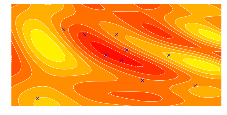
The next point is taken as the maximizer of l(x)/g(x), as shown in the figure below:
Tree-structured Parzen estimator optimization in action. Brown crosses below indicate the 10 samples on which EI is evaluated, which are sampled from the Parzen density estimator of the good group. Notice the lower exploration strategy compared to the Gaussian process.
The tree structure mentioned in the name of the method is linked to the structure of the Parzen estimators. As the hyper-parameters are tree-structured (see discussion above), so are the Parzen estimators which are simple kernel density estimators. One of the great drawbacks of tree-structured Parzen estimators is that they do not model interactions between the hyper-parameters. It is thus much less able than Gaussian processes when two hyper-parameters strongly interact.
Algorithms dedicated to hyper-parameter tuning
Here are algorithms which were developed specifically for hyper-parameter tuning.
The two following methods (Hyperband and PBT) introduce a form of early stopping for bad runs. For all the previous methods, each learning has to be run until the end.
Hyperband
Hyperband is a variation of random search, but with some explore-exploittheory to find the best time allocation for each of the configurations. It is described in details in [9]. A good introduction to this algorithm is the successive halving algorithm:
- Randomly sample 64 hyper-parameter sets in the search space.
- Evaluate after 100 iterations the validation loss of all these.
- Discard the lowest performers of them to keep only a half.
- Run the good ones for 100 iterations more and evaluate.
- Discard a half.
- Run the good ones for 200 iterations more and evaluate.
- Repeat till you have only one model left.
This algorithm needs a definition of an iteration (can be set so that the first model evaluation is done after a couple of epochs) and a total budget of iterations (which will set the total number of explored configurations).
Successive halving suffers from what is called the “n vs B/n” trade-off in [9]. Bis the total budget to be allocated for hyper-parameter search, and n is the number of configurations to be explored. B/n is the average amount of resource allocated to a specific configuration.
For a given budget, it is not clear whether to search for many configurations (large n) for a small time, or explore few configurations but allocating a lot of resources to them (large B/n). For a given problem, if hyper-parameter configurations can be discriminated quickly (if the dataset converges fast, if bad configurations reveal themselves quickly, or if the hyper-parameter search space is not chosen wisely enough so that a randomly picked one is likely to be very bad), then n should be chosen large. On the contrary, if they are slow to differentiate (or if the search space is small, but the best configuration is sought with high confidence), then B/n should be large (at the expense of the number of tested configurations).
The drawbacks of these strategies are the following:
- If n is large, then some good configurations which can be slow to converge at the beginning will be killed off early.
- If B/n is large, then bad configurations will be given a lot of resources, even though they could have been stopped before.
Hyperband does away with this dilemma by considering several possible values of n for a fixed B, in essence performing a grid search over feasible value of n [9].
In the infinite time limit, this enables to find the optimal allocation strategy.
In [9], it is shown on some real world tests that a simple successive halving with a correct balance of n vs B/n is very competitive against Hyperband (and in many cases better), though it might not generalize for every problem.
On a more practical point, using Hyperband means that you are able to checkpoint your model during learning, so that it can be stopped and resumed.
PBT (Population-based training)
Population-based training mixes ideas from genetic optimization algorithms during the SGD optimization steps. The learning of the ML model is seen as a dynamical system where hyper-parameters are to be chosen every p time steps. The algorithm is described in [7], with a broad overview on the blog post of the authors.
The idea is the following: take k agents, each of them are given a model to train, randomly sampled from the search space.
After p learning iterations, do the exploit phase of the algorithm:
- each of the worker compares itself to the other workers (either all of them, a random subset of them, or only one randomly chosen).
- If the validation performance of the worker is significantly worse (in a statistical meaning) than the best of the others, the worker copies both the hyper-parameters and the weights of the best performing model
- if the worker has changed its model, do the explore phase of the algorithm, i.e. perturb the hyper-parameters before restarting to learn (several strategies exist: for some randomly chosen hyper-parameters, re-sample them randomly from the search space or perturb them all by a multiplicative coefficient between e.g. 0.8 and 1.2)
Loop the algorithm by relearning for p iterations.
At the end of your training time budget, take the best performing model.
It should be noted that the algorithm is asynchronous: workers do not need to wait for the others to complete their p learning iterations. They can compare their performance to current state of the other models.
The size of the population should be large enough to sufficiently explore the hyper-parameter space and lower the variance of the population.
This algorithm blends together the hyper-parameter search with the learning, so that it only produces a model at the end, and not a hyper-parameter configuration. For instance, if one uses PBT to optimize the learning rate, the algorithm finds a good learning rate schedule. If one selects the final hyper-parameters of the best model and relearns a model from scratch using this, the model is expected to have subpar performance (see figure 5.d and paragraph 4.4, Hyperparameter Adaptivity in [7]). Is some sense, PBT find a (locally) optimal learning schedule.
A side effect of weight sharing during the exploit phase means that hyper-parameters pertaining to model shape or structure (i.e. number of neurons in a layer, size of the hashing space for logistic regression, etc.) cannot be tuned by PBT.
Fabolas
Fabolas, standing for fast Bayesian optimization for large datasets, described in [8] tries to increase the speed of Bayesian optimization by learning the ML model on a sampled dataset (but evaluating its performance on the full validation dataset). The idea is that a small portion of the data (less than 10 %) is sufficient to check if a hyper-parameter combination is promising or not.
To do it efficiently, it adds another parameter, continuous from 0 to 1, which sets the fraction of the dataset on which to learn the model. It involves a complex acquisition function (which is derived from entropy search, which is an acquisition function based on the predicted information gain around the optimum) and a special covariance kernel.
BOHB
BOHB (Bayesian Optimization and HyperBand) mixes the Hyperband algorithm and Bayesian optimization. It is described in [3] and also in this blog post. It uses Hyperband to determine how many configurations to try within a budget but instead of randomly sampling them, it uses a Bayesian optimizer (using a Parzen estimator with no tree structure).
At the beginning of the run, it uses Hyperband capability to sample many configurations with a small budget to explore quickly and efficiently the hyper-parameter search space and get very soon promising configurations, but uses the Bayesian optimizer predictive power to propose good configurations close to the optimum.
It is also parallel (as Hyperband) which overcomes a strong short-coming of Bayesian optimization.
Conclusion
Choosing the right hyper-parameter optimization algorithm depends on the ML problem, the computing infrastructure and the associated computing budget, etc. A random search might be sufficient if the ML model is very simple and can be run fast, but it will not be efficient enough for large scale ML models. Using Hyperband (or its associated algorithm BOHB) means that the ML model can be checkpointed during training. PBT aims at finding an optimal training schedule rather than optimizing the hyper-parameters.
References
[1] ^ Bergstra, James S., Rémi Bardenet, Yoshua Bengio, and Balázs Kégl. “Algorithms for hyper-parameter optimization.” In Advances in neural information processing systems, pp. 2546–2554. 2011.
[2] ^ Bergstra, James, and Yoshua Bengio. “Random search for hyper-parameter optimization.” Journal of Machine Learning Research 13, no. Feb (2012): 281–305.
[3] ^ Falkner, Stefan, Aaron Klein, and Frank Hutter. “BOHB: Robust and efficient hyperparameter optimization at scale.” arXiv preprint arXiv:1807.01774 (2018).
[4] ^¹ ^² Franceschi, Luca, Michele Donini, Paolo Frasconi, and Massimiliano Pontil. “Forward and reverse gradient-based hyperparameter optimization.” In Proceedings of the 34th International Conference on Machine Learning-Volume 70, pp. 1165–1173. JMLR. org, 2017.
[5] ^ Garrido-Merchán, Eduardo C., and Daniel Hernández-Lobato. “Dealing with Integer-valued Variables in Bayesian Optimization with Gaussian Processes.” arXiv preprint arXiv:1706.03673 (2017).
[6] ^ Ginsbourger, David, Rodolphe Le Riche, and Laurent Carraro. “Kriging is well-suited to parallelize optimization.” In Computational intelligence in expensive optimization problems, pp. 131–162. Springer, Berlin, Heidelberg, 2010.
[7] ^¹ ^² Jaderberg, Max, Valentin Dalibard, Simon Osindero, Wojciech M. Czarnecki, Jeff Donahue, Ali Razavi, Oriol Vinyals et al. “Population based training of neural networks.” arXiv preprint arXiv:1711.09846 (2017).
[8] ^ Klein, Aaron, Stefan Falkner, Simon Bartels, Philipp Hennig, and Frank Hutter. “Fast bayesian optimization of machine learning hyperparameters on large datasets.” arXiv preprint arXiv:1605.07079 (2016)
[9] ^¹ ^² Li, Lisha, Kevin Jamieson, Giulia DeSalvo, Afshin Rostamizadeh, and Ameet Talwalkar. “Hyperband: A novel bandit-based approach to hyperparameter optimization.” arXiv preprint arXiv:1603.06560 (2016).
[10] ^ Maclaurin, Dougal, David Duvenaud, and Ryan Adams. “Gradient-based hyperparameter optimization through reversible learning.” In International Conference on Machine Learning, pp. 2113–2122. 2015.
[11] ^¹ ^² C. E. Rasmussen & C. K. I. Williams, Gaussian Processes for Machine Learning, the MIT Press, 2006,ISBN 026218253X, link to full book in pdf
[12] ^ Wilson, James, Frank Hutter, and Marc Deisenroth. “Maximizing acquisition functions for Bayesian optimization.” In Advances in Neural Information Processing Systems, pp. 9906–9917. 2018.
Author: Aloïs Bissuel