
FOCS is one of the top two conferences in theoretical computer science (according to Wikipedia). It has a long history: this year’s edition was the 59th! It has been known with its current name since 1975.
It assembles a fairly small community of theoretical computer scientists — I heard around 260 people registered. It is organized with mainly two parallel sessions of 20 minutes talks for 3 days (see program).
As a machine learning scientist, theory of computer science is not my area of specialty and it was my first time attending. I was positively impressed by the quality of the talks. They covered a wide range of algorithms, and even though the focus was on proving bounds, the presenters made a wonderful job of giving intuitions and core ideas rather than theorem upon theorem. The typical talk structure would include:
– a usually pedagogical introduction to the problem of interest, including necessary definitions, and very often intuitions or toy problems for illustration, and applications,
– an overview of the history of the problem, or at least background and previous work (or rather, previous bounds),
– the outline of the proposed algorithm, specifying the most important tools used,
– a sketch of the proof,
– a conclusion with open problems.
Even though no-one showed experimental results, i.e. involving real-world data, most often the algorithms were shown to have practical applications — from dynamic pricing to image denoising. I found the presentations introduced a number of tools which I think might help in either understanding or improving our current algorithms dealing with large-scale, high-dimensional data. In the following paragraphs, I’ll detail few papers that stood out from my point of view.
How do you optimize search in high-dimensions?
In Contextual Search via Intrinsic Volumes, the authors consider the problem of contextual multi-dimensional binary search, where the goal is to find the value of a vector [latex]v \in [0, 1]^d[/latex]. At each round,
– an adversary provides a context [latex]u_t \in \mathbb{R}^d[/latex],
– the learner guesses a value [latex]p_t[/latex],
– the learner incurs a loss [latex]\ell(\langle u_t, v\rangle, p_t)[/latex],
– and learns whether or not [latex]p_t \leq \langle u_t, v\rangle[/latex].
The goal of the learner is then to minimize their total loss [latex]\sum_{t=1}^T \ell(\langle u_t, v\rangle, p_t)[/latex].
The strategy in the case [latex]d=1[/latex] is trivial, you just have to split a segment in half at each step. In the where [latex]d=2[/latex], the natural strategy is to divide in half the search area. In the worst case, though, where the area is “long and skinny”, using the perimeter is better, so that in general, using a strategy based on decreasing a potential function [latex]\phi(S_t) = \text{perimeter}(S_t) + \sqrt{\text{area}(S_t)}[/latex] has better regret.
They generalize from the 2D case to higher dimensions by relying on intrinsic volumes, which are well studied in integral geometry. Formally, intrinsic volumes are defined as the coefficients that arise in Steiner’s formula of the volume of the sum of a convex set [latex]K\subseteq\mathbb{R}^d[/latex] and a unit ball [latex]B[/latex]:
[latex] \text{Vol}(K + \varepsilon B) = \sum_{j=0}^d \kappa_{d-j} V_j(K) \varepsilon^{d-j},[/latex]
where [latex]V_j(K)[/latex] are the normalized coefficients of the polynomial and [latex]\kappa_{d-j}[/latex] is the volume of the [latex](d-j)[/latex]-dimensional unit ball.
Building upon the set of elegant properties previously shown for these volumes, the authors are able to provide an algorithm that achieves regret [latex]O(\mathtt{poly}(d))[/latex] for the case of minimizing a loss [latex]\ell(\theta, p)=|\theta – p|[/latex], where previous best-known algorithms incurred regret [latex]O(\mathtt{poly}(d)\log(T))[/latex].
How do you efficiently estimate densities for large datasets?
Rajesh Jayaram presented an algorithm to do Perfect [latex]L_p[/latex] Sampling in a Data Stream. Sampling has been shown very useful in the statistical analysis of large data streams.
Given a stream of updates to the coordinates of a vector [latex]f\in\mathbb{R}^n[/latex], an approximate [latex]L_p[/latex] sampler must output, after a single pass, an index [latex]i^*\in[n][/latex] such that for every [latex]j\in[n][/latex],
[latex]P(i^*=j) =\frac{|f_j|^p}{||f||_p^p}(1\pm\nu) + O(n^{-c}),[/latex]
where :
– [latex]c\ge1[/latex] is an arbitrarily large constant,
– [latex]\nu\in[0,1)[/latex] is the relative error
– the sampler is allowed to output [latex]\texttt{FAIL}[/latex] with probability [latex]\delta[/latex],
– a stream of updates for [latex]f\in\mathbb{R}^n[/latex] is given as [latex]f_i \leftarrow f_i + \Delta[/latex], where [latex]\Delta[/latex] can be positive or negative case.
When [latex]\nu=0[/latex], the sampler is said to be perfect.
In the case where [latex]p=1[/latex] and [latex]\Delta>0[/latex], the problem is easily solved using [latex]O(\log n)[/latex] bits of space with reservoir sampling.
The authors demonstrate the existence of a perfect [latex]L_p[/latex]-sampler for the case [latex]p\in(0,2)[/latex]. The main idea is based on improving precision sampling. The classical samplers usually follow the same pattern:
1. perform a linear transformation of [latex]z_i = f_i/t_i^{1/p}[/latex].
2. Run count-sketch on [latex]z[/latex] to estimate [latex]y[/latex].
3. Find [latex]i^*=\arg\max_i|y_i|[/latex]. Run a statistical test to decide whether to output [latex]i^*[/latex] or [latex]y[/latex].
Instead of using a linear transformation of the inputs based on uniform random variables [latex]t_i[/latex], they scale the inputs with exponential random variables, which have nicer properties, namely for scaling: if [latex]t_i \sim \exp(1)[/latex], then [latex]t_i/f_i \sim \exp(f_i)[/latex]. They exploit previous observations on the distribution of the anti-rank vector [latex](D(1), D(2), \dots, D(n))[/latex], where [latex]D(k)\in[n][/latex] is a random variable which gives the index of the [latex]t[/latex]-th smallest exponential of [latex](t_1, \dots, t_n)[/latex] independently distributed exponentials, eg for any [latex]k\in[n][/latex]:
[latex]t_{D(k)} = \sum_{i=1}^k \frac{E_i}{\sum_{j=i}^n \lambda_{D(j)}},[/latex]
where the [latex]E_i[/latex] are iid exponential variables with mean [latex]1[/latex] and independent of the anti-rank vector.
Paris Siminelakis presented a new algorithm for Efficient Density Evaluation for Smooth Kernels. Kernel density estimation is a well known non-parametric problem, with many applications in machine learning. At its core lies the necessity of computing the kernel density function of a dataset [latex]P\subset \mathbb{R}^d[/latex], defined for a point [latex]x\in\mathbb{R}^d[/latex] as:
[latex]KDF_P(x):=\frac{1}{|P|}\sum_{y\in P}k(x,y).[/latex]
This problem is notoriously hard to solve in practice, since this function needs to be evaluated quickly, for a large dataset [latex]P[/latex] and many points [latex]x[/latex], and often in high-dimension.
The authors build on the previous techniques: (a) partitioning the data space and split the estimate in a set of “smaller” kernels — typically with methods such as quad-trees, thus hard to scale to high dimensions (exponential dependence), and (b) using importance sampling through hashing — requiring a specific hashing scheme, and requiring a number of samples which can grow large through a dependence on the minimum of the kernel, i.e. [latex]\mu[/latex] such that [latex]KDF_P(x)\geq\mu[/latex]. Describing the algorithm they present would not fit in a short summary, but in a nutshell, the idea is to build quad-trees on a random projection of the input space, use reservoir sampling in each cell to provide a partition estimator of the density.
Another interesting presentation was from Manolis Zampetakis, presenting Efficient Statistics, in High Dimensions, from Truncated Samples — generalizing the early results from Galton, 1897, to multivariate truncated normal estimation. One of their main results is to prove that without access to an oracle indicating whether a sample belongs to the truncated set, it is impossible to approximate the unknown normal.
How do you sample in graphs?
Many presentations tackled graph algorithms. The definition of the graph Laplacian came up in several presentations, in different flavors.
The authors of A Matrix Chernoff Bound for Strongly Rayleigh Distributions and Spectral Sparsifiers from a few Random Spanning Trees introduce a new matrix concentration bound to show guarantees on the computation of spectral sparsifiers of graph Laplacians through sums of random spanning trees. There is a history of results on concentration bounds for sums of random variables, among which the Chernoff bound is one of the most popular. The authors propose to study the concentration of measure for matrix-valued random variables, and derived a Matrix Chernoff bound for [latex]k[/latex]-homogeneous Strongly Rayleigh Distributions. They use this bound to compute concentration bounds for sums of Laplacians of independent random spanning trees, and draw conclusions on graph sparsification. Interestingly, their proof uses Doob martingales, i.e. martingales built from sequences of conditional expectations, which have nice mathematical properties.
A very different work uses random-walk based sampling. In Sublinear algorithms for local graph centrality estimation, the authors focus on the PageRank and Heat Kernel definitions of centrality and show a how to build a “perfect” estimator for [latex]P(v)[/latex] with good approximation guarantees and how to avoid expanding “heavy” nodes in the random walk, while keeping these guarantees.
Knuth Prize
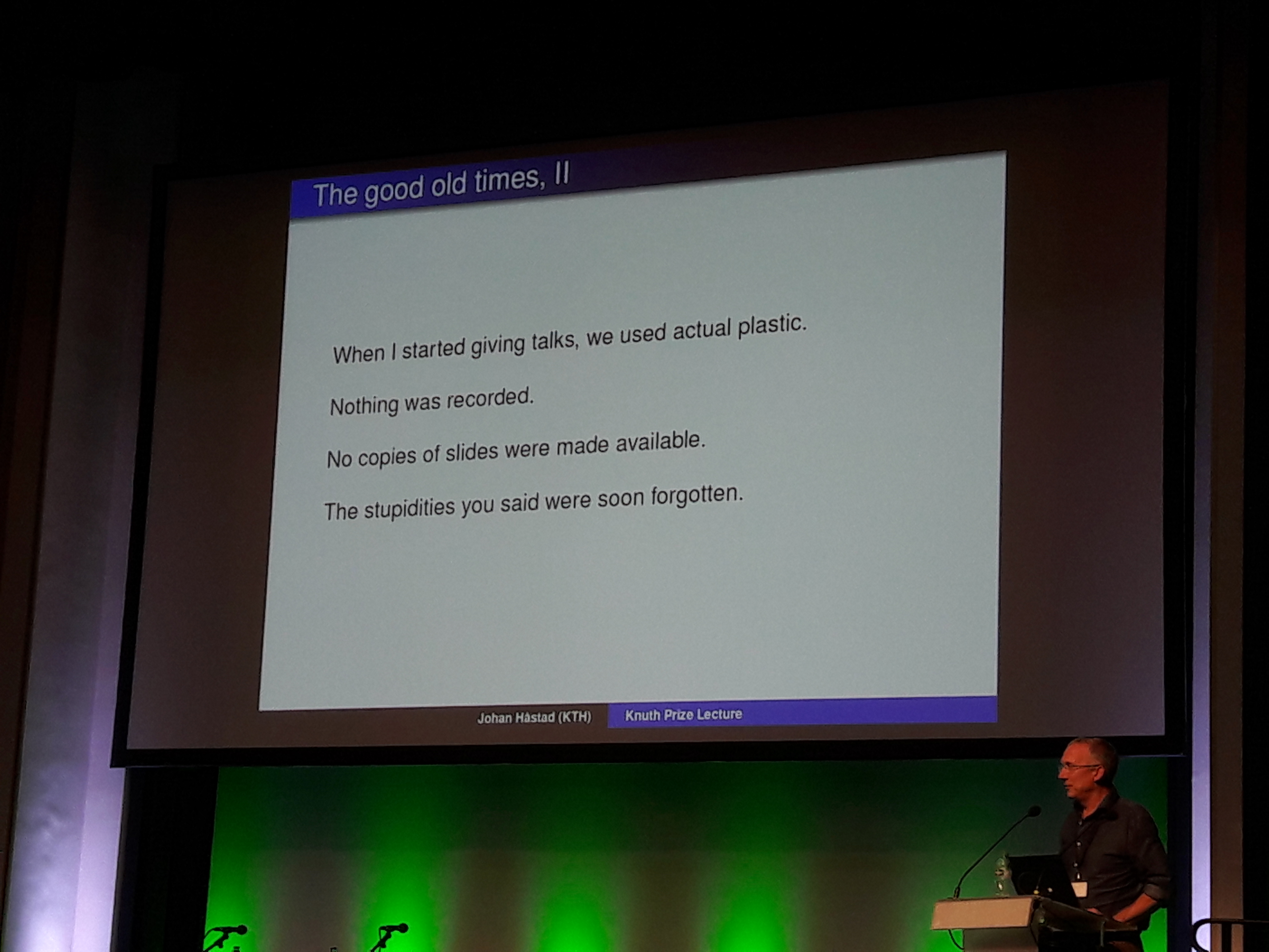
Johan Håstad giving the Knuth Prize lecture
It is worth mentioning that the last talk on Monday 8th was the Knuth Prize Lecture by this year’s winner, Johan Håstad. He shared “random thoughts”, looking back to his career, with some advice — such as knowing the right people at the right time and moving around to increase chances for luck to strike. I didn’t understand much of the technical part, except that he seemed to admire the PCP theorem a lot, and he said that working on the Unique Games Conjecture was a good idea. Always good to know :-).
Conclusion
Even though it’s not always clear how applicable the results are in practice, I found it interesting to note the recurring patterns: sketching, random projections, trees, sampling, hashing… As we are already using some of these principles to handle the large scale of data we deal with everyday at Criteo, getting to grips with the underlying theory and seeing how the different techniques work together was pure fuel for ideas.
Post written by:
 |
| Anne-Marie Tousch, Machine Learning Scientist, Criteo AI Lab |