
Data filtering for reliable decision making. Photo credit: Getty-images
In this post we present our data-driven approach to design a relevant filter for ABTest result analysis…
Criteo Engine consists of distinct components (bidder, recommender system, banner renderer, marketplace, …) that together handle bid requests in real-time all the way to delivering personalized ad banners. Every week the Engine is subject to modifications proposed by our R&D teams. Whenever a proposal has made its way up to online testing, it usually undergoes the following process:
- AB-Test the proposed modification against the reference engine in production.
- After the ABTest is finished, compute a business metric M over the ABTest scope. Usually M= difference of clients’ business value between populations A and B.
- Check whether 0 falls into the outside-left region of the metrics confidence interval, in order to decide whether the tested engine change is an improvement or not.
Useful data for decision making are unfortunately sparse…
As long as we consider metrics related to rich signals (e.g. displays or clicks), we generally end up with fairly good metric estimates with small confidence intervals. But when it comes to sparser signals such as total sales or total order-value generated to our clients –which are those that truly matter from a business perspective–, problems come into sight: the confidence interval amplitude becomes larger (typically 5 to 10 times larger than for rich aforementioned signals) and as a result the ABTest is too often declared “inconclusive”.
Filtering data helps…
To cope with that issue, the usual solution is to remove noise by applying filters on the sparse signal. For instance, excluding or capping abnormally large values, and/or using business-specific filters such as, for instance, removing all sales from users who could not have been exposed to any ad (i.e. without any bid in the period preceding the sale). Generally speaking, what we expect from a good filter is, removing useless signal –the so-called noise—by trading off bias against variance.
Now, there are a bunch of candidate filters to denoise a signal, with parameters to fine-tune, and the question is, how to select the best one?
Our filter selection principles…
Rather than optimizing an explicit bias-variance tradeoff typically using confidence interval sizes –which is convenient to compute but not always aligned with business criteria–, we directly focus on what we are primarily interested in: maximizing the overall rate of good decision-making (regarding the underlying-but-unknown ground truth).
For that purpose we have setup a simulation framework to be able to compute the so-called decision-error-rate of the candidate filter at hand, namely, the probability of wrong decisions when using the given candidate filter (see figure 1 below). Within our simulation framework, this probability is estimated through a series of repeated randomized experiments where each time the ground truth is known (we control the overall difference of business metric between populations A and B when generating simulation data).
 Figure 1: The graph represents the overall decision-error-rate when using a given candidate filter. the X-axis represents values of simulated business-metric differences between populations A and B. The Y-axis gives the corresponding decision-error-rate, namely, the probability that 0 falls into our filtered-metric confidence interval whereas the underlying business metric difference has positive value. |
Another complementary criterion that we compute to summarize the performance into one unique number is the so-called minimum-noticeable-difference, defined as the smallest underlying difference (in %) in business metric between A and B that the candidate filter is able to detect with decision-error-rate no more than 5%. Figure 2 below summarizes the interplay between these two main criteria.
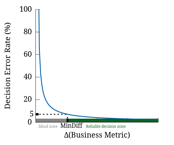 Figure 2: When fixing an upper-bound (here 5%) on the decision-error-rate (Y-axis), we have a related X-axis value, the so-called Minimum-Noticeable-Difference (MinDiff), namely the smallest difference between populations A and B that can be reliably detected by our metric. |
And the winner is…
Running those repeated simulations extensively for a bunch of candidate filters and using MinDiff to rank them, we finally found that the best way to denoise our data for the purpose of post-ABTest decision-making is, combining abnormal-user removal (those with largest business metric values) with “sales-without-preceding-bid” removal. Our evaluation framework enabled us to both select those two filters and fine-tune their respective parameter values.
Post written by:
 Regis Vert |
 Thomas Ricatte |