
In computational advertising, evaluating click-through rate (CTR) is one of the most important tasks. The most widely used model for CTR prediction is called logistic regression, which learns a model [latex]\boldsymbol{w}[/latex] by solving the following optimization problem.
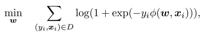
where [latex]\boldsymbol{x}_i[/latex] is an impression, [latex]y_i \in \{1, -1\}[/latex] is the label, and [latex]D[/latex] is the training set. Here, [latex]\phi(\boldsymbol{w}, \boldsymbol{x}) = \boldsymbol{w} \cdot \boldsymbol{x}[/latex] is called a linear model. In this post, I will explain that linear models are not suitable for learning feature conjunctions, which is an important functionality for the problem of CTR prediction. I will then introduce three models that learn feature conjunctions, and explain their differences.
To get started, say we have two features Publisher and Advertiser, and some ad impressions from NIKE displayed on ESPN:

For the linear model, [latex]\phi(\boldsymbol{w}, \boldsymbol{x}) = w_{\text{ESPN}} + w_{\text{NIKE}}[/latex], which means we will learn a weight for ESPN and another weight for NIKE. Conceptually, these two weights learn the average behavior of ESPN and NIKE, respectively. Therefore, if the CTR of the ads from NIKE on ESPN is particularly high or low, we will not learn this effect well.
Degree-2 Polynomial Mappings (Poly2)
To learn the effect of a feature conjunction, the most naive way is to learn a dedicated weight for it. This model is called degree-2 polynomial mapping (Poly2). In our example: [latex]\phi(\boldsymbol{w}, \boldsymbol{x}) = w_{\text{ESPN},\text{NIKE}} [/latex].
Note that this post focuses on modelling feature conjunctions, so we ignore the linear terms. You can easily add them back if you want: [latex]\phi(\boldsymbol{w}, \boldsymbol{x}) = w_{\text{ESPN}} + w_{\text{NIKE}} + w_{\text{ESPN},\text{NIKE}}[/latex].
The problem of Poly2 is that when the data is sparse, there may be some unseen pairs in the test set. In this case, Poly2 will make trivial prediction on those unseen pairs.
Factorization Machines (FMs)
To address this problem, Steffen Rendle proposed factorization machines (FMs), a method that learns the feature conjunction in a latent space. In FMs, each feature has an associated latent vector, and the conjunction of any two features is modelled by the inner-product of two latent vectors. Back to our example, we now have: [latex]\phi(\boldsymbol{w}, \boldsymbol{x}) = \boldsymbol{w}_{\text{ESPN}} \cdot \boldsymbol{w}_{\text{NIKE}}[/latex].
The benefit of FMs is that in the case of predicting on unseen data from the test set, we may still be able to do a reasonable prediction. Consider the following data set:
 We see that there are no (ESPN, Gucci) pairs in the training data. For Poly2, there is no way to learn the weight [latex]w_{\text{ESPN},\text{Gucci}}[/latex]. However, for FMs, we may still be able to do reasonable predictions because we can learn [latex]\boldsymbol{w}_{\text{ESPN}}[/latex] from (ESPN, NIKE) pairs and [latex]\boldsymbol{w}_{\text{Gucci}}[/latex] from (Vogue, Gucci) pairs.
Field-aware Factorization Machines (FFMs)
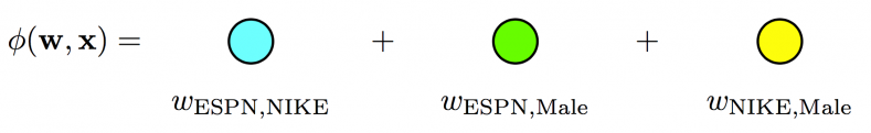
Before introducing our last model, Field-aware Factorization Machines (FFMs), let us add one more feature to our previous example:
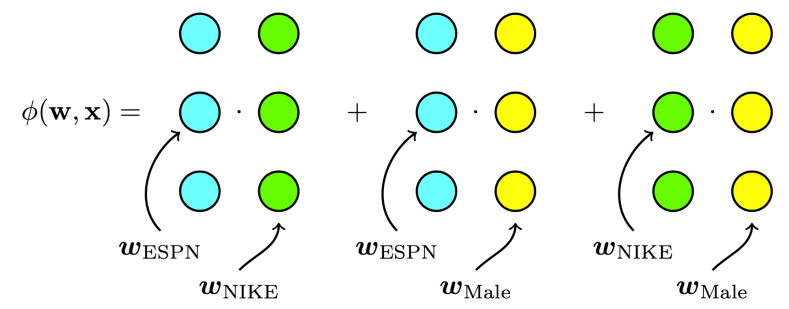
 In this example, for FM, we have:
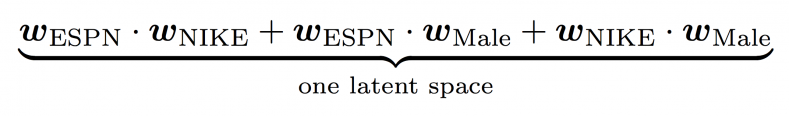
We see that in the case of FMs, there is only one latent space, which means each feature has only one latent vector, and this latent vector is used to interact with any other latent vectors from other features. Take ESPN as an example, [latex]{\boldsymbol w}_{\text{ESPN}}[/latex] is used to learn the latent effect with NIKE ([latex]{\boldsymbol w}_{\text{ESPN}} \cdot {\boldsymbol w}_{\text{NIKE}}[/latex]) and Male ([latex]{\boldsymbol w}_{\text{ESPN}} \cdot {\boldsymbol w}_{\text{Male}}[/latex]).
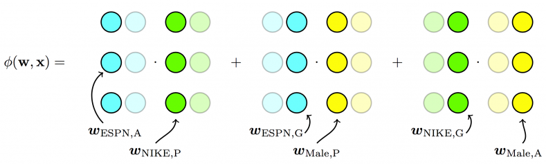
The idea of FFMs is to split the original latent space into many “smaller” latent spaces, and depending on the fields of features, one of them is used. In our example, there are three latent spaces: Publisher (P) × Advertiser (A), Publisher (P) × Gender (G), and Advertiser (A) × Gender (G). Since the latent effect between publishers and advertisers may be very different from the latent effect between publishers and gender, it may be better to split them than to mix them. Now, [latex]\phi({\boldsymbol w}, {\boldsymbol x})[/latex] becomes:
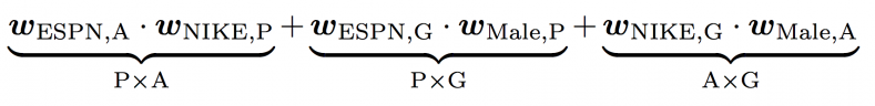
We see that to learn the latent effect of (ESPN, NIKE), [latex]{\boldsymbol w}_{\text{ESPN}, \text{A}}[/latex] is used because NIKE belongs to the field Advertiser, and [latex] {\boldsymbol w}_{\text{NIKE}, \text{P}}[/latex] is used because ESPN belongs to the field Publisher. Again, to learn the latent effect of (EPSN, Male), [latex]{\boldsymbol w}_{\text{ESPN}, \text{G}}[/latex] is used because Male belongs to the field Gender, and [latex]{\boldsymbol w}_{\text{Male}, \text{P}}[/latex] is used because ESPN belongs to the field Publisher.
The difference between Poly2, FMs, and FFMs is illustrated in the following figures.
- For Poly2, a dedicated weight is learned for each feature pair:
- For FMs, each feature has one latent vector, which is used to interact with any other latent vectors:
- For FFMs, each feature has several latent vectors, one of them is used depending on the field of the other feature:
FFMs have been used to win the first prize of three CTR competitions hosted by Criteo, Avazu, Outbrain, and also the third prize of RecSys Challenge 2015.
Two related papers are available:
- Field-aware Factorization Machines for CTR Prediction
- Field-aware Factorization Machines in a Real-world Online Advertising System
Finally, if you want to use FFM, you can find an implementation here:
https://github.com/guestwalk/libffm